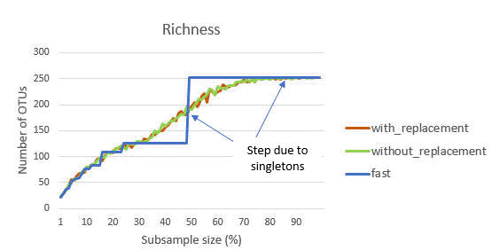
Jagged steps in the fast rarefaction curve
See also
Rarefaction
alpha_div_rare command
The figure below shows the rarefaction curve for richness for a typical sample as generated by the alpha_div_rare command . There are three calculation methods: fast, with replacement and without replacement (see otutab_subsample command for description of the methods).
With the fast approximation, the count for an OTU is multiplied by the subsample fraction (e.g., 0.5 for 50%) and rounded to the nearest integer. If this count is zero, the OTU is not included. If the fraction is <0.5, then an OTU with a total count of 1 will be rounded to zero. This explains the step between <50% and >50% that is seen in the fast curve: these are singleton counts that are excluded <50% and included >50%. Similarly, there is a step at 1/4 = 25% due to OTUs with a count of 2, at 1/6 = 16% for OTUs with a count of 3 and so on.
These steps are not seen when using randomized sub-sampling with or without replacement. These curves show a smoother convergence towards a horizontal asymptote. In traditional diversity analysis, this would be interpreted as indicating that most OTUs in the community have been observed and few new OTUs would be found with additional sampling effort. However, this is not a valid conclusion with UPARSE or UNOISE OTUs because low-abundance reads are discarded, which causes singletons and other low-abundance OTUs to be underrepresented in individual samples. On the other hand, if low-abundance reads are retained, then the rarefaction curve will not converge because low-abundance spurious OTUs will continue to be created as new reads are added. Rarefaction curves are therefore hard / impossible to interpret regardeless of whether low-abundance reads or OTUs are discarded, and in my opinion rarefaction analysis has little value with NGS OTUs.


